Part 1: Basic Concepts

Bias-Variance Tradeoff
Underfitting vs. Overfitting
Ensemble Methods
Loss Functions
Confusion Matrix
- Accuracy
- Recall
- Precision
ROC Curves, PR Curves

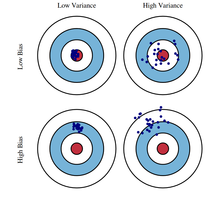
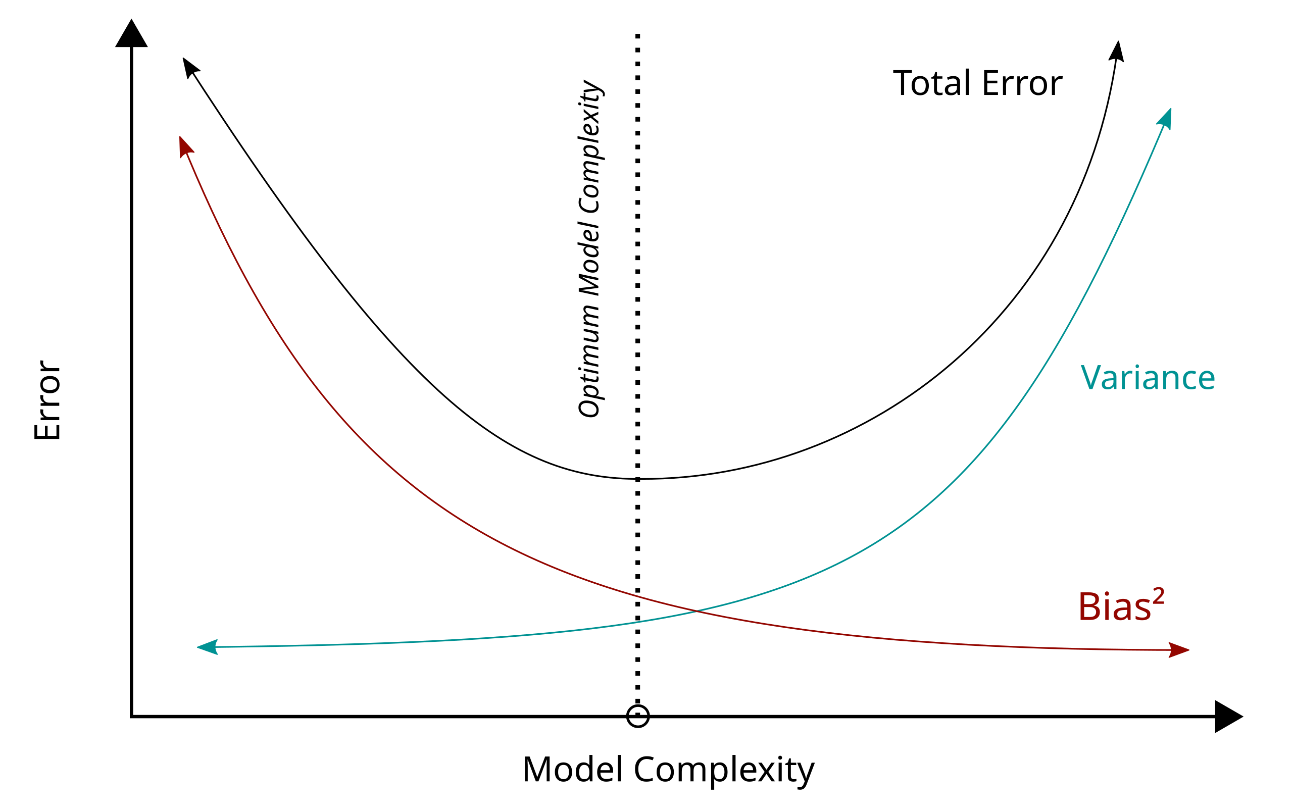
Bias-Variance Tradeoff

Decomposition of Expected Test Error:

$$ \begin{align*} \underbrace{\mathbb{E}_{x, y, D} \left[ \left( h_D(x) - y \right)^2 \right]}_{\text{Expected Test Error}} &= \underbrace{\mathbb{E}_{x, D} \left[ \left( h_D(x) - \bar{h}(x) \right)^2 \right]}_{\text{Variance}} + \underbrace{\mathbb{E}_{x, y} \left[ \left( \bar{y}(x) - y \right)^2 \right]}_{\text{Noise}} + \underbrace{\mathbb{E}_x \left[ \left( \bar{h}(x) - \bar{y}(x) \right)^2 \right]}_{\text{Bias}^2} \end{align*} $$

Variance: How "over-specialized" (overfitting) is your classifier to a particular training set?
Bias: What is the inherent error that you obtain from your classifier even with infinite training data?
- Inherent to model
Noise: How big is the data-intrinsic noise?
- Inherent to data

Underfitting vs. Overfitting

Characteristic	Overfitting	Underfitting
Training Error	Low	High
Validation/Test Error	High	High
Model Complexity	Too complex	Too simple
Generalization	Poor	Poor
Bias vs. Variance	Low bias, high variance	High bias, low variance

Cross-Validation

Algorithm
1. Split the dataset into k-folds (e.g., 5 or 10)
2. Train the model on $k-1$ folds and validate it on the remaining fold
3. Repeat the process $k$ times, rotating the validation fold each time
4. Compute the average training and validation errors across all folds
Model Generalization Evaluation
- Low training error and high validation error → Overfitting
- High training error and high validation error → Underfitting
- Similar and low training and validation errors → Good generalization

Fixing High Bias (Underfitting)

Increase Model Complexity
Decrease Regularization
Add Features
Increase Training Time
Use Non-linear Models

Fixing High Variance (Overfitting)

Decrease Model Complexity
Increase Regularization
Reduce Feature Space
Increase Training Data
Use Early Stopping
Use Ensemble Methods

Balance: Bias-Variance Tradeoff

The solution often lies in striking a balance between high bias and high variance. You can experiment iteratively with:

Model selection: Trying different algorithms and architectures
Hyperparameter tuning: Adjusting hyperparameters like learning rate, regularization strength, or model depth
Feature engineering: Improving the input data to enhance model performance

Ensemble Methods

Pros & Cons

(+) Improved accuracy/predictive performance
(+) Improved robustness to overfitting and noisy data
(+) Flexibility to use different types of models
(-) Increased complexity (requires more computational resources)
(-) Harder to interpret compared to a single model

1. Bagging (Bootstrap Aggregating)

Combines bootstrapping with aggregation
- Bootstrapping is a statistical technique used to generate multiple datasets by randomly sampling (with replacement) from the original dataset
- Each bootstrapped dataset is the same size as the original dataset but may contain duplicate samples
Reduces variance

2. Boosting

Training weak learners sequentially to correct errors from the previous one
Reduces bias

3. Stacking (Stacked Generalization)

Improves predictive power by combining predictions from multiple models
A meta-model is trained on the outputs of base models

Ensemble Algorithms

Random Forest: Bagging applied to decision trees
AdaBoost: Boosting algorithm that combines decision trees or stumps
Gradient Boosting Machines (GBM): Sequential training to minimize loss
XGBoost, LightGBM, CatBoost: Optimized implementations of gradient boosting with faster training and improved accuracy

Loss functions

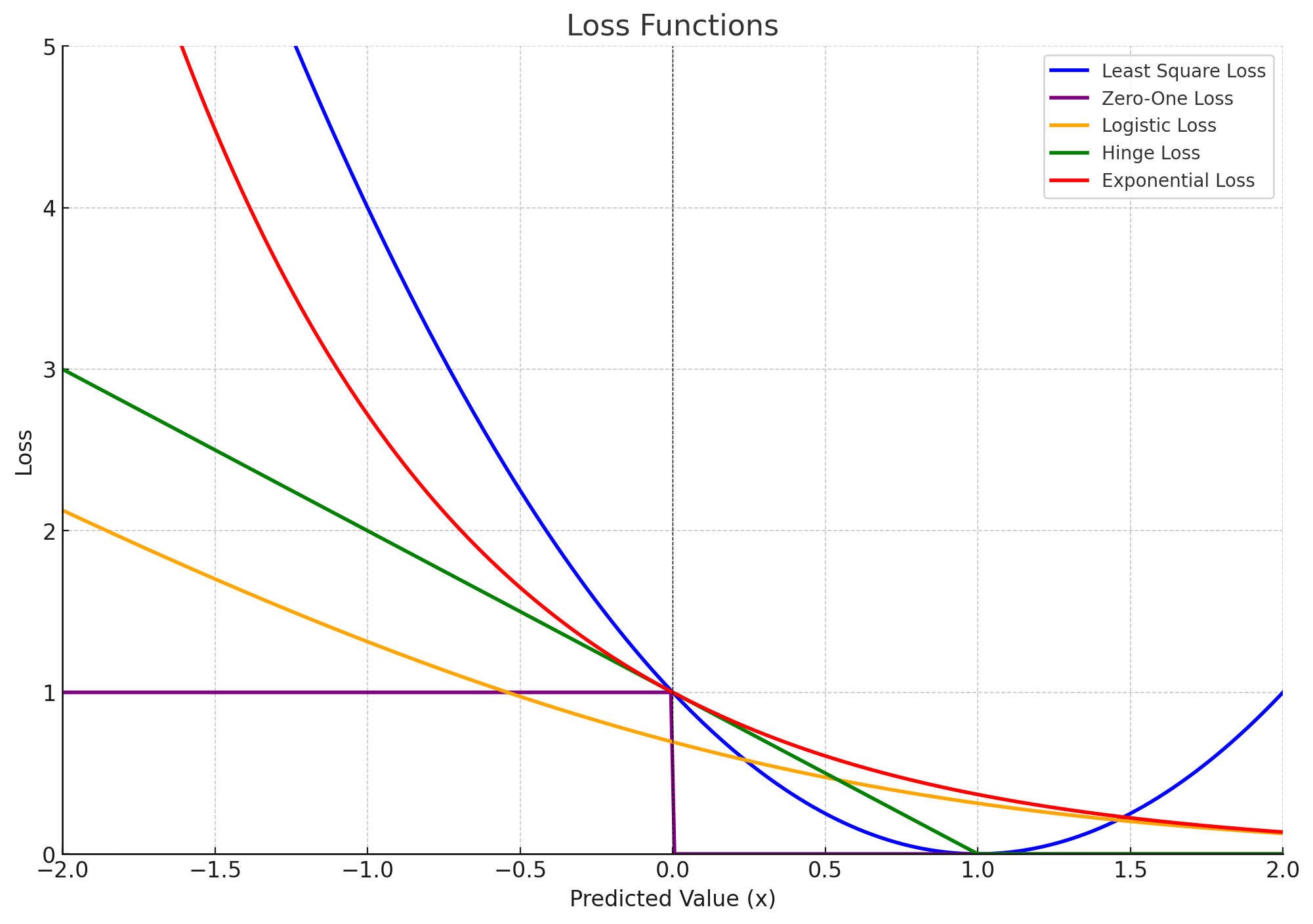
Loss functions provide a mathematical framework to quantify the error between a model's predictions and the true labels.

$h_\theta(x)$: Predicted value (or raw model output, i.e. logits) for a given input $x$
- $h$: The hypothesis function (i.e., the model)
- $\theta$: Model parameters (e.g., weights, biases) learned during training
- $x$: Input features (a single data point or a feature vector)
$y$: True value (or ground truth) corresponding to the input $x$

Loss Functions for Classification

Least Square Loss: $(h_\theta(x) - y)^2$
- Smooth and differentiable
- Highly affected by outliers
Zero-One Loss: $1{h_\theta(x) \cdot y \leq 0}$
- Rarely used in practice; Non-smooth and difficult to optimize using gradient descent
- Least sensitive to outliers
Logistic Loss: $\log(1 + \exp(-h_\theta(x) \cdot y))$
- Smooth and differentiable, suitable for optimization using gradient descent
- Commonly used in logistic regression for binary classification when $y \in {-1, 1}$
- Operates on predicted score (logit) ($h_\theta(x)$) without applying an activation function
Hinge Loss: $\max{1 - h_\theta(x) \cdot y, 0}$
- Smooth and differentiable, suitable for optimization using gradient descent
- Commonly used for SVMs to maximize the margins
Exponential Loss: $\exp(-h_\theta(x) \cdot y)$
- Smooth and differentiable, suitable for optimization using gradient descent
- Commonly used in boosting algorithms like AdaBoost
Cross-Entropy Loss:
- Smooth and differentiable, suitable for optimization using gradient descent
- Operates on probabilities ($\hat{y}$), which are derived from the logits using an activation function (e.g., sigmoid or softmax)
- Used for both binary and multiclass classification
  - For binary classification: $-[y \log(\hat{y}) + (1 - y) \log(1 - \hat{y})]$
    - $y \in {0, 1}$
    - $\hat{y}$ is the predicted probability (output of a sigmoid function)
  - For multiclass classification: $-\sum_{i=1}^C y_i \log(\hat{y}_i)$
    - $C$ is the number of classes
    - $y_i$ is the true label (one-hot encoded)
    - $\hat{y}_i$ is the predicted probability (output of a softmax function)

Loss Functions for Regression

Root Mean Square Error (RMSE): $RMSE = \sqrt{\frac{1}{n} \sum_{j=1}^n (y_i - \hat{y}_i)^2}$
- Gives higher weight to large errors, useful when large errors are particularly undesirable
Mean Absolute Error (MAE): $MAE = \frac{1}{n} \sum_{i=1}^n |y_i - \hat{y}_i|$
- Measures the average magnitude of errors without squaring
- Provides a steady metric unaffected by extreme values
RMSE vs. MAE:
- RMSE is always greater than or equal to MAE; If all errors are equal, RMSE = MAE
- MAE is easier to interpret

MLE vs. Loss Functions

MLE (Maximum Likelihood Estimation) derives loss functions for probabilistic models by:
- maximizing the likelihood of the observed data
- minimizing the negative log-likelihood
Loss functions are broader and can be used for tasks beyond probability models (e.g., regression, classification)

Batch Learning vs. Online Learning

Batch Learning:
- Learns from all the available training data at once
Online Learning:
- Learns gradually, processing one example (or a small batch) at a time as data becomes available
- Error-driven approach, where the model adjusts itself after each new example is received
- Examples
  - Stock market prediction
  - Email classification
  - Recommendation systems
  - Ad placement in a new market
- Algorithm
  - Goal: Minimize the number of mistakes made by the model over time
  - The process is iterative and works as follows:
    1. Receive an unlabeled instance $x^{(i)}$
    2. Predict the output $y' = h_\theta(x^{(i)})$
    3. Receive the true label $y^{(i)}$
    4. Suffer a loss if the prediction $y' \neq y^{(i)}$
    5. Update the parameters $\theta$ to reduce future mistakes

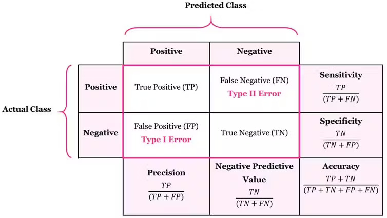
Confusion Matrix

	Predicted Positive	Predicted Negative
True Positive	TP	FN
True Negative	FP	TN

Accuracy: $(TP + TN) / \text{all}$
- Measures how many cases (both positive and negative) are correctly classified
Recall (Sensitivity/True Positive Rate): $TP / (TP + FN)$
- Measures how many actual positive cases are correctly classified
- Sensitive to imbalanced data
Precision: $TP / (TP + FP)$
- Measures how many predicted positive cases are actually correct


High Recall, Low Precision	Many false positives but few false negatives	Good for detection
Low Recall, High Precision	Few false positives but many false negatives	Good for trustworthiness

F1 Score: $2 \cdot \frac{\text{recall } \cdot \text{ precision}}{\text{recall } + \text{ precision}}$
- Harmonic mean of recall and precision, useful for imbalanced datasets
Specificity (True Negative Rate): $TN / (TN + FP)$
- Measures the ability to correctly classify negatives

Severity of False Positives vs. False Negatives:
- False Positives are worse in cases like:
  - Non-contagious diseases (unnecessary treatment)
  - HIV tests (psychological impact)
- False Negatives are worse in cases like:
  - Early treatment importance
  - Quality control defects
  - Software testing (critical errors missed)

ROC Curves, PR Curves

ROC (Receiver Operating Characteristic) Curves

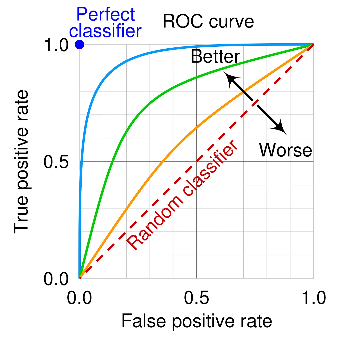
ROC curve plots recall (TPR) vs. 1 - specificity (FPR)
AUC (Area Under the Curve):
- AUC near 1 indicates a good model
- AUC near 0.5 indicates a model performing like random guessing

Precision-Recall Curves

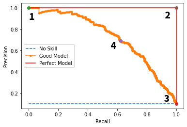
PR curves are preferred when the dataset is highly imbalanced or when the focus is on the minority class detection
Ignores true negatives; Used when classifier specificity is not a concern
AUC-PR (Area Under the PR Curve):
- A higher AUC-PR indicates better performance
- Point 1: Low Recall, High Precision
- Point 2: Perfect model
- Point 3: High Recall, Low Precision
- Point 4: Trade-off